An introduction to causal graphs and how to use them

Causal graphs are graphical objects that attach causal notions to each edge and missing edge. We will review some of the fundamental causal graphs used in causal inference, and their differences from traditional graphs.

import networkx as nx
import numpy as np
import pandas as pd
from dowhy import gcm
from dowhy.gcm.util.general import set_random_seed
from scipy import stats

import pywhy_graphs
import pywhy_graphs.networkx as pywhy_nx
from pywhy_graphs import CPDAG, PAG
from pywhy_graphs.viz import draw

Structural Causal Models: Simulating some data

Structural causal models (SCMs) [1] are mathematical objects defined by a 4-tuple <V, U, F, P(U)>, where:

• V is the set of endogenous observed variables

• U is the set of exogenous unobserved variables

• F is the set of functions for every $v in V$

• P(U) is the set of distributions for all $u in U$

Taken together, these four objects define the generating causal mechanisms for a causal problem. Almost always, the SCM is not known. However, the SCM induces a causal graph, which has nodes from V and then edges are defined by the arguments of the functions in F. If there are common exogenous parents for any V, then this can be represented in an Acyclic Directed Mixed Graph (ADMG), or a causal graph with bidirected edges. The common latent confounder is represented with a bidirected edge between two endogenous variables.

Even though the SCM is typically unknown, we can still use it to generate ground-truth simulations to evaluate various algorithms and build our intuition. Here, we will simulate some data to understand causal graphs in the context of SCMs.

# set a random seed to make example reproducible
seed = 12345
rng = np.random.RandomState(seed=seed)


class MyCustomModel(gcm.PredictionModel):
    def __init__(self, coefficient):
        self.coefficient = coefficient

    def fit(self, X, Y):
        # Nothing to fit here, since we know the ground truth.
        pass

    def predict(self, X):
        return self.coefficient * X

    def clone(self):
        # We don't really need this actually.
        return MyCustomModel(self.coefficient)


# set a random seed to make example reproducible
set_random_seed(1234)

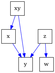
# construct a causal graph that will result in
# xy - > x -> y <- z -> w
#  \_________/^
G = nx.DiGraph([("x", "y"), ("z", "y"), ("z", "w"), ("xy", "x"), ("xy", "y")])
dot_graph = draw(G)
dot_graph.render(outfile="dag.png", view=True)

causal_model = gcm.ProbabilisticCausalModel(G)
causal_model.set_causal_mechanism("xy", gcm.ScipyDistribution(stats.binom, p=0.5, n=1))
causal_model.set_causal_mechanism("z", gcm.ScipyDistribution(stats.binom, p=0.9, n=1))
causal_model.set_causal_mechanism(
    "y",
    gcm.AdditiveNoiseModel(
        prediction_model=MyCustomModel(1),
        noise_model=gcm.ScipyDistribution(stats.binom, p=0.8, n=1),
    ),
)
causal_model.set_causal_mechanism(
    "w",
    gcm.AdditiveNoiseModel(
        prediction_model=MyCustomModel(1),
        noise_model=gcm.ScipyDistribution(stats.binom, p=0.5, n=1),
    ),
)
causal_model.set_causal_mechanism(
    "x",
    gcm.AdditiveNoiseModel(
        prediction_model=MyCustomModel(1),
        noise_model=gcm.ScipyDistribution(stats.binom, p=0.5, n=1),
    ),
)

# Fit here would not really fit parameters, since we don't do anything in the fit method.
# Here, we only need this to ensure that each FCM has the correct local hash (i.e., we
# get an inconsistency error if we would modify the graph afterwards without updating
# the FCMs). Having an empty data set is a small workaround, since all models are
# pre-defined.
gcm.fit(causal_model, pd.DataFrame(columns=["x", "y", "z", "w", "xy"]))

# sample the observational data
data = gcm.draw_samples(causal_model, num_samples=500)

print(data.head())
print(pd.Series({col: data[col].unique() for col in data}))

# note the graph shows colliders, which is a collision of arrows
# for example between ``x`` and ``z`` at ``y``.
draw(G)

Fitting causal models:   0%|          | 0/5 [00:00<?, ?it/s]
Fitting causal mechanism of node x:   0%|          | 0/5 [00:00<?, ?it/s]
Fitting causal mechanism of node y:   0%|          | 0/5 [00:00<?, ?it/s]
Fitting causal mechanism of node z:   0%|          | 0/5 [00:00<?, ?it/s]
Fitting causal mechanism of node w:   0%|          | 0/5 [00:00<?, ?it/s]
Fitting causal mechanism of node xy:   0%|          | 0/5 [00:00<?, ?it/s]
Fitting causal mechanism of node xy: 100%|██████████| 5/5 [00:00<00:00, 954.29it/s]
   z  xy  w  x  y
0  1   1  1  1  1
1  1   1  2  2  3
2  1   1  2  1  2
3  1   0  2  0  1
4  1   0  2  0  1
z           [1, 0]
xy          [1, 0]
w        [1, 2, 0]
x        [1, 2, 0]
y     [1, 3, 2, 0]
dtype: object

<graphviz.graphs.Digraph object at 0x7fd529d98b90>

Causal Directed Ayclic Graphs (DAG): Also known as Causal Bayesian Networks

Causal DAGs represent Markovian SCMs, also known as the “causally sufficient” assumption, where there are no unobserved confounders in the graph.

print(G)

# One can query the parents of 'y' for example
print(list(G.predecessors("y")))

# Or the children of 'x'
print(list(G.successors("xy")))

# Using the graph, we can explore d-separation statements, which by the Markov
# condition, imply conditional independences.
# For example, 'z' is d-separated from 'x' because of the collider at 'y'
print(f"'z' is d-separated from 'x': {nx.d_separated(G, {'z'}, {'x'}, set())}")

# Conditioning on the collider, opens up the path
print(f"'z' is d-separated from 'x' given 'y': {nx.d_separated(G, {'z'}, {'x'}, {'y'})}")

DiGraph with 5 nodes and 5 edges
['x', 'z', 'xy']
['x', 'y']
/home/circleci/project/examples/intro/intro_causal_graphs.py:140: DeprecationWarning: d_separated is deprecated and will be removed in NetworkX v3.5.Please use `is_d_separator(G, x, y, z)`.
  print(f"'z' is d-separated from 'x': {nx.d_separated(G, {'z'}, {'x'}, set())}")
'z' is d-separated from 'x': True
/home/circleci/project/examples/intro/intro_causal_graphs.py:143: DeprecationWarning: d_separated is deprecated and will be removed in NetworkX v3.5.Please use `is_d_separator(G, x, y, z)`.
  print(f"'z' is d-separated from 'x' given 'y': {nx.d_separated(G, {'z'}, {'x'}, {'y'})}")
'z' is d-separated from 'x' given 'y': False

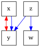
Acyclic Directed Mixed Graphs (ADMG)

ADMGs represent Semi-Markovian SCMs, where there are possibly unobserved confounders in the graph. These unobserved confounders are graphically depicted with a bidirected edge.

# We can construct an ADMG from the DAG by just setting 'xy' as a latent confounder
admg = pywhy_graphs.set_nodes_as_latent_confounders(G, ["xy"])

# Now there is a bidirected edge between 'x' and 'y'
dot_graph = draw(admg)
dot_graph.render(outfile="admg.png", view=True)

# Now if one queries the parents of 'y', it will not show 'xy' anymore
print(list(admg.predecessors("y")))

# The bidirected edges also form a cluster in what is known as "confounded-components", or
# c-components for short.
print(f"The ADMG has confounded-components: {list(admg.c_components())}")

# We can also look at m-separation statements similarly to a DAG.
# For example, 'z' is still m-separated from 'x' because of the collider at 'y'
print(f"'z' is d-separated from 'x': {pywhy_nx.m_separated(admg, {'z'}, {'x'}, set())}")

# Conditioning on the collider, opens up the path
print(f"'z' is d-separated from 'x' given 'y': {pywhy_nx.m_separated(admg, {'z'}, {'x'}, {'y'})}")

# Say we add a bidirected edge between 'z' and 'x', then they are no longer
# d-separated.
admg.add_edge("z", "x", admg.bidirected_edge_name)
print(
    f"'z' is d-separated from 'x' after adding a bidirected edge z<->x: "
    f"{pywhy_nx.m_separated(admg, {'z'}, {'x'}, set())}"
)

# Markov Equivalence Classes
# --------------------------
#
# Besides graphs that represent causal relationships from the SCM, there are other
# graphical objects used in the causal inference literature.
#
# Markov equivalence class graphs are graphs that encode the same Markov equivalences
# or d-separation statements, or conditional independences. These graphs are commonly
# used in constraint-based structure learning algorithms, which seek to reconstruct
# parts of the causal graph from data. In this next section, we will briefly overview
# some of these common graphs.
#
# Markov equivalence class graphs are usually learned from data. The algorithms for
# doing so are in `dodiscover <https://github.com/py-why/dodiscover>`_. For more
# details on causal discovery (i.e. structure learning algorithms), please see that repo.

['z', 'x']
The ADMG has confounded-components: [{'y', 'x'}, {'z'}, {'w'}]
'z' is d-separated from 'x': True
'z' is d-separated from 'x' given 'y': False
'z' is d-separated from 'x' after adding a bidirected edge z<->x: False

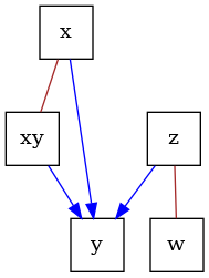
Completed Partially Directed Ayclic Graph (CPDAG)

CPDAGs are Markov Equivalence class graphs that encode the same d-separation statements as a causal DAG that stems from a Markovian SCM. All relevant variables are assumed to be observed. An uncertain edge orientation is encoded via a undirected edge between two variables. Here, we’ll construct a CPDAG that encodes the same d-separations as the earlier DAG.

Typically, CPDAGs are learnt using some variant of the PC algorithm [2].

cpdag = CPDAG()

# let's assume all the undirected edges are formed from the earlier DAG
cpdag.add_edges_from(G.edges, cpdag.undirected_edge_name)

# next, we will orient all unshielded colliders present in the original DAG
cpdag.orient_uncertain_edge("x", "y")
cpdag.orient_uncertain_edge("xy", "y")
cpdag.orient_uncertain_edge("z", "y")

dot_graph = draw(cpdag)
dot_graph.render(outfile="cpdag.png", view=True)

'cpdag.png'

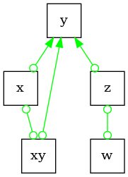
Partial Ancestral Graph (PAG)

PAGs are Markov equivalence classes for ADMGs. Since we allow latent confounders, these graphs are more complex compared to the CPDAGs. PAGs encode uncertain edge orientations via circle endpoints. A circle endpoint (o-*) can imply either: a tail (-*), or an arrowhead (<-*), which can then imply either an undirected edge (selection bias), directed edge (ancestral relationship), or bidirected edge (possible presence of a latent confounder).

Typically, PAGs are learnt using some variant of the FCI algorithm [2] and [3].

pag = PAG()

# let's assume all the undirected edges are formed from the earlier DAG
for u, v in nx.Graph(G.edges).edges:
    pag.add_edge(u, v, pag.circle_edge_name)
    pag.add_edge(v, u, pag.circle_edge_name)

# next, we will orient all unshielded colliders present in the original DAG
pag.orient_uncertain_edge("x", "y")
pag.orient_uncertain_edge("xy", "y")
pag.orient_uncertain_edge("z", "y")

dot_graph = draw(pag)
dot_graph.render(outfile="pag.png", view=True)

'pag.png'

References

[1]

Judea Pearl. Causality: Models, Reasoning and Inference. Cambridge University Press, USA, 2nd edition, 2009. ISBN 052189560X.

[2] (1,2)

Peter Spirtes, Clark Glymour, and Richard Scheines. Causation, Prediction, and Search. Volume 81. The MIT Press, 01 1993. ISBN 978-1-4612-7650-0. doi:10.1007/978-1-4612-2748-9.

[3]

Jiji Zhang. On the completeness of orientation rules for causal discovery in the presence of latent confounders and selection bias. Artificial Intelligence, 172(16):1873–1896, 2008. URL: https://www.sciencedirect.com/science/article/pii/S0004370208001008, doi:https://doi.org/10.1016/j.artint.2008.08.001.

Estimated memory usage: 252 MB