Demo for the DoWhy causal API

We show a simple example of adding a causal extension to any dataframe.

import dowhy.datasets
import dowhy.api
from dowhy.graph import build_graph_from_str

import numpy as np
import pandas as pd

from statsmodels.api import OLS

data = dowhy.datasets.linear_dataset(beta=5,
        num_common_causes=1,
        num_instruments = 0,
        num_samples=1000,
        treatment_is_binary=True)
df = data['df']
df['y'] = df['y'] + np.random.normal(size=len(df)) # Adding noise to data. Without noise, the variance in Y|X, Z is zero, and mcmc fails.
nx_graph = build_graph_from_str(data["dot_graph"])

treatment= data["treatment_name"][0]
outcome = data["outcome_name"][0]
common_cause = data["common_causes_names"][0]
df

	W0	v0	y
0	-0.330622	False	0.887729
1	-0.691849	False	-1.118670
2	0.193915	False	-0.966624
3	-0.535931	True	2.642023
4	2.334936	True	7.962068
...	...	...	...
995	0.339981	False	-0.948675
996	-0.919134	False	0.069790
997	-1.140944	False	-0.716580
998	0.352853	True	4.586724
999	-0.983083	True	6.705248

1000 rows × 3 columns

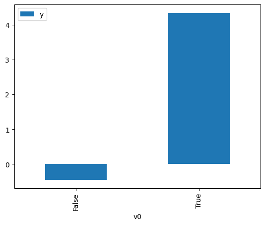
# data['df'] is just a regular pandas.DataFrame
df.causal.do(x=treatment,
             variable_types={treatment: 'b', outcome: 'c', common_cause: 'c'},
             outcome=outcome,
             common_causes=[common_cause],
            ).groupby(treatment).mean().plot(y=outcome, kind='bar')

<Axes: xlabel='v0'>

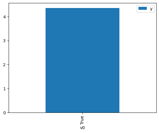
df.causal.do(x={treatment: 1},
              variable_types={treatment:'b', outcome: 'c', common_cause: 'c'},
              outcome=outcome,
              method='weighting',
              common_causes=[common_cause]
              ).groupby(treatment).mean().plot(y=outcome, kind='bar')

<Axes: xlabel='v0'>

cdf_1 = df.causal.do(x={treatment: 1},
              variable_types={treatment: 'b', outcome: 'c', common_cause: 'c'},
              outcome=outcome,
              graph=nx_graph
              )

cdf_0 = df.causal.do(x={treatment: 0},
              variable_types={treatment: 'b', outcome: 'c', common_cause: 'c'},
              outcome=outcome,
              graph=nx_graph
              )

cdf_0

	W0	v0	y	propensity_score	weight
0	-0.416171	False	-1.103170	0.587029	1.703494
1	1.020597	False	1.610446	0.256853	3.893284
2	0.289512	False	1.261112	0.415118	2.408955
3	-0.807504	False	-1.508775	0.676307	1.478619
4	-0.127578	False	0.523608	0.516908	1.934579
...	...	...	...	...	...
995	0.193915	False	-0.966624	0.438129	2.282434
996	-0.663361	False	-1.209901	0.644508	1.551571
997	0.507649	False	-0.926918	0.364117	2.746373
998	1.261393	False	0.781840	0.214268	4.667049
999	-1.187408	False	-1.447086	0.752270	1.329309

1000 rows × 5 columns

cdf_1

	W0	v0	y	propensity_score	weight
0	-1.096630	True	1.579037	0.264752	3.777119
1	0.883869	True	6.774463	0.716633	1.395414
2	-1.335124	True	2.590650	0.221639	4.511850
3	-1.064736	True	4.180466	0.270908	3.691296
4	-0.712749	True	2.574438	0.344435	2.903306
...	...	...	...	...	...
995	-0.394069	True	4.852584	0.418255	2.390889
996	-2.109866	True	-0.132723	0.117258	8.528192
997	1.342959	True	7.022089	0.798937	1.251663
998	0.263952	True	3.750980	0.578761	1.727828
999	-1.284152	True	2.070227	0.230414	4.340014

1000 rows × 5 columns

Comparing the estimate to Linear Regression

First, estimating the effect using the causal data frame, and the 95% confidence interval.

(cdf_1['y'] - cdf_0['y']).mean()

$\displaystyle 4.86323421622536$

1.96*(cdf_1['y'] - cdf_0['y']).std() / np.sqrt(len(df))

$\displaystyle 0.141690908498881$

Comparing to the estimate from OLS.

model = OLS(np.asarray(df[outcome]), np.asarray(df[[common_cause, treatment]], dtype=np.float64))
result = model.fit()
result.summary()

OLS Regression Results

Dep. Variable:	y	R-squared (uncentered):	0.921
Model:	OLS	Adj. R-squared (uncentered):	0.921
Method:	Least Squares	F-statistic:	5840.
Date:	Wed, 06 Dec 2023	Prob (F-statistic):	0.00
Time:	08:43:32	Log-Likelihood:	-1436.2
No. Observations:	1000	AIC:	2876.
Df Residuals:	998	BIC:	2886.
Df Model:	2
Covariance Type:	nonrobust

	coef	std err	t	P>|t|	[0.025	0.975]
x1	1.1002	0.028	39.374	0.000	1.045	1.155
x2	4.9739	0.050	99.704	0.000	4.876	5.072

Omnibus:	0.374	Durbin-Watson:	1.968
Prob(Omnibus):	0.829	Jarque-Bera (JB):	0.380
Skew:	0.047	Prob(JB):	0.827
Kurtosis:	2.984	Cond. No.	1.79

Notes:
[1] R² is computed without centering (uncentered) since the model does not contain a constant.
[2] Standard Errors assume that the covariance matrix of the errors is correctly specified.