Estimating effect of multiple treatments#
[1]:
from dowhy import CausalModel
import dowhy.datasets

import warnings
warnings.filterwarnings('ignore')
[2]:
data = dowhy.datasets.linear_dataset(10, num_common_causes=4, num_samples=10000,
                                     num_instruments=0, num_effect_modifiers=2,
                                     num_treatments=2,
                                     treatment_is_binary=False,
                                     num_discrete_common_causes=2,
                                     num_discrete_effect_modifiers=0,
                                     one_hot_encode=False)
df=data['df']
df.head()
[2]:
| X0 | X1 | W0 | W1 | W2 | W3 | v0 | v1 | y | |
|---|---|---|---|---|---|---|---|---|---|
| 0 | 0.504656 | 0.967232 | -0.970066 | -2.217805 | 2 | 1 | -4.162334 | -4.536053 | -45.392428 |
| 1 | 0.775272 | 0.411631 | 0.646069 | -1.206054 | 0 | 0 | -2.270521 | 0.449863 | -24.278870 |
| 2 | -0.880358 | -1.475509 | -0.400533 | 0.258120 | 2 | 2 | 14.910592 | 3.347291 | -30.063886 |
| 3 | 0.277932 | 0.314129 | -0.068397 | -1.114949 | 3 | 1 | 10.073269 | 3.658561 | 175.000075 |
| 4 | -2.218957 | -0.645205 | -0.120087 | -0.740175 | 0 | 0 | -3.975991 | -4.182782 | -158.147502 |
[3]:
model = CausalModel(data=data["df"],
                    treatment=data["treatment_name"], outcome=data["outcome_name"],
                    graph=data["gml_graph"])
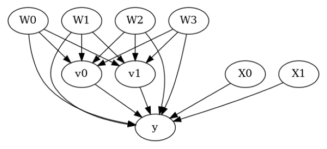
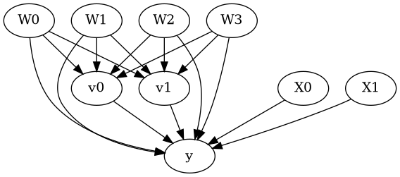
[4]:
model.view_model()
from IPython.display import Image, display
display(Image(filename="causal_model.png"))
[5]:
identified_estimand= model.identify_effect(proceed_when_unidentifiable=True)
print(identified_estimand)
Estimand type: EstimandType.NONPARAMETRIC_ATE

### Estimand : 1
Estimand name: backdoor
Estimand expression:
    d
─────────(E[y|W2,W1,W0,W3])
d[v₀  v₁]
Estimand assumption 1, Unconfoundedness: If U→{v0,v1} and U→y then P(y|v0,v1,W2,W1,W0,W3,U) = P(y|v0,v1,W2,W1,W0,W3)

### Estimand : 2
Estimand name: iv
No such variable(s) found!

### Estimand : 3
Estimand name: frontdoor
No such variable(s) found!
Linear model#
Let us first see an example for a linear model. The control_value and treatment_value can be provided as a tuple/list when the treatment is multi-dimensional.
The interpretation is change in y when v0 and v1 are changed from (0,0) to (1,1).
[6]:
linear_estimate = model.estimate_effect(identified_estimand,
                                        method_name="backdoor.linear_regression",
                                        control_value=(0,0),
                                        treatment_value=(1,1),
                                        method_params={'need_conditional_estimates': False})
print(linear_estimate)
*** Causal Estimate ***

## Identified estimand
Estimand type: EstimandType.NONPARAMETRIC_ATE

### Estimand : 1
Estimand name: backdoor
Estimand expression:
    d
─────────(E[y|W2,W1,W0,W3])
d[v₀  v₁]
Estimand assumption 1, Unconfoundedness: If U→{v0,v1} and U→y then P(y|v0,v1,W2,W1,W0,W3,U) = P(y|v0,v1,W2,W1,W0,W3)

## Realized estimand
b: y~v0+v1+W2+W1+W0+W3+v0*X0+v0*X1+v1*X0+v1*X1
Target units: ate

## Estimate
Mean value: 25.979841502154613
You can estimate conditional effects, based on effect modifiers.
[7]:
linear_estimate = model.estimate_effect(identified_estimand,
                                        method_name="backdoor.linear_regression",
                                        control_value=(0,0),
                                        treatment_value=(1,1))
print(linear_estimate)
*** Causal Estimate ***

## Identified estimand
Estimand type: EstimandType.NONPARAMETRIC_ATE

### Estimand : 1
Estimand name: backdoor
Estimand expression:
    d
─────────(E[y|W2,W1,W0,W3])
d[v₀  v₁]
Estimand assumption 1, Unconfoundedness: If U→{v0,v1} and U→y then P(y|v0,v1,W2,W1,W0,W3,U) = P(y|v0,v1,W2,W1,W0,W3)

## Realized estimand
b: y~v0+v1+W2+W1+W0+W3+v0*X0+v0*X1+v1*X0+v1*X1
Target units:

## Estimate
Mean value: 25.979841502154613
### Conditional Estimates
__categorical__X0  __categorical__X1
(-3.776, -0.776]   (-3.101, -0.194]     11.079653
                   (-0.194, 0.397]      16.318110
                   (0.397, 0.89]        19.601416
                   (0.89, 1.484]        22.437455
                   (1.484, 4.885]       27.590046
(-0.776, -0.2]     (-3.101, -0.194]     15.383771
                   (-0.194, 0.397]      20.403288
                   (0.397, 0.89]        23.340525
                   (0.89, 1.484]        26.486628
                   (1.484, 4.885]       31.760537
(-0.2, 0.321]      (-3.101, -0.194]     17.709720
                   (-0.194, 0.397]      22.911817
                   (0.397, 0.89]        25.921107
                   (0.89, 1.484]        29.108866
                   (1.484, 4.885]       34.218027
(0.321, 0.891]     (-3.101, -0.194]     20.066997
                   (-0.194, 0.397]      25.370238
                   (0.397, 0.89]        28.390558
                   (0.89, 1.484]        31.561974
                   (1.484, 4.885]       36.636974
(0.891, 3.851]     (-3.101, -0.194]     24.532166
                   (-0.194, 0.397]      29.585736
                   (0.397, 0.89]        32.514156
                   (0.89, 1.484]        35.856095
                   (1.484, 4.885]       40.702137
dtype: float64
More methods#
You can also use methods from EconML or CausalML libraries that support multiple treatments. You can look at examples from the conditional effect notebook: https://py-why.github.io/dowhy/example_notebooks/dowhy-conditional-treatment-effects.html
Propensity-based methods do not support multiple treatments currently.