Demo for the DoWhy causal API#
We show a simple example of adding a causal extension to any dataframe.
[1]:
import dowhy.datasets
import dowhy.api
from dowhy.graph import build_graph_from_str

import numpy as np
import pandas as pd

from statsmodels.api import OLS
[2]:
data = dowhy.datasets.linear_dataset(beta=5,
        num_common_causes=1,
        num_instruments = 0,
        num_samples=1000,
        treatment_is_binary=True)
df = data['df']
df['y'] = df['y'] + np.random.normal(size=len(df)) # Adding noise to data. Without noise, the variance in Y|X, Z is zero, and mcmc fails.
nx_graph = build_graph_from_str(data["dot_graph"])

treatment= data["treatment_name"][0]
outcome = data["outcome_name"][0]
common_cause = data["common_causes_names"][0]
df
[2]:
| W0 | v0 | y | |
|---|---|---|---|
| 0 | -1.092232 | False | -1.467122 |
| 1 | -0.553488 | True | 5.092333 |
| 2 | -2.721292 | False | 0.557821 |
| 3 | -0.860433 | False | -0.864048 |
| 4 | -1.078330 | True | 3.316149 |
| ... | ... | ... | ... |
| 995 | -1.934879 | False | -0.464891 |
| 996 | -0.240524 | False | -0.196877 |
| 997 | -1.365115 | False | 1.737968 |
| 998 | -1.312072 | False | -0.211613 |
| 999 | -2.285569 | False | -2.284761 |
1000 rows × 3 columns
[3]:
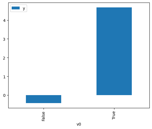
# data['df'] is just a regular pandas.DataFrame
df.causal.do(x=treatment,
             variable_types={treatment: 'b', outcome: 'c', common_cause: 'c'},
             outcome=outcome,
             common_causes=[common_cause],
            ).groupby(treatment).mean().plot(y=outcome, kind='bar')
[3]:
<Axes: xlabel='v0'>
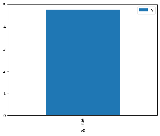
[4]:
df.causal.do(x={treatment: 1},
              variable_types={treatment:'b', outcome: 'c', common_cause: 'c'},
              outcome=outcome,
              method='weighting',
              common_causes=[common_cause]
              ).groupby(treatment).mean().plot(y=outcome, kind='bar')
[4]:
<Axes: xlabel='v0'>
[5]:
cdf_1 = df.causal.do(x={treatment: 1},
              variable_types={treatment: 'b', outcome: 'c', common_cause: 'c'},
              outcome=outcome,
              graph=nx_graph
              )

cdf_0 = df.causal.do(x={treatment: 0},
              variable_types={treatment: 'b', outcome: 'c', common_cause: 'c'},
              outcome=outcome,
              graph=nx_graph
              )
[6]:
cdf_0
[6]:
| W0 | v0 | y | propensity_score | weight | |
|---|---|---|---|---|---|
| 0 | -0.762795 | False | -1.106836 | 0.741823 | 1.348030 |
| 1 | -0.639424 | False | -1.569639 | 0.713176 | 1.402178 |
| 2 | 0.270371 | False | 0.446674 | 0.461197 | 2.168270 |
| 3 | -1.889006 | False | 0.264200 | 0.914941 | 1.092967 |
| 4 | -0.732039 | False | 0.578589 | 0.734859 | 1.360806 |
| ... | ... | ... | ... | ... | ... |
| 995 | -2.200991 | False | 1.705738 | 0.939414 | 1.064493 |
| 996 | 0.338915 | False | -0.224639 | 0.441305 | 2.266005 |
| 997 | -0.556969 | False | -0.198539 | 0.693007 | 1.442988 |
| 998 | -1.732231 | False | 0.170568 | 0.899507 | 1.111720 |
| 999 | -0.504828 | False | -0.317645 | 0.679853 | 1.470905 |
1000 rows × 5 columns
[7]:
cdf_1
[7]:
| W0 | v0 | y | propensity_score | weight | |
|---|---|---|---|---|---|
| 0 | -0.687302 | True | 3.268349 | 0.275483 | 3.629985 |
| 1 | -1.452541 | True | 5.436494 | 0.134246 | 7.449006 |
| 2 | -0.978979 | True | 4.749862 | 0.212678 | 4.701941 |
| 3 | -0.397370 | True | 5.544810 | 0.348158 | 2.872257 |
| 4 | 0.406560 | True | 5.071772 | 0.578143 | 1.729677 |
| ... | ... | ... | ... | ... | ... |
| 995 | -0.943522 | True | 5.675177 | 0.219720 | 4.551243 |
| 996 | -1.128276 | True | 6.212309 | 0.184846 | 5.409895 |
| 997 | 0.130132 | True | 6.075339 | 0.497787 | 2.008891 |
| 998 | 0.092802 | True | 4.321617 | 0.486851 | 2.054015 |
| 999 | -0.357319 | True | 4.093820 | 0.358886 | 2.786397 |
1000 rows × 5 columns
Comparing the estimate to Linear Regression#
First, estimating the effect using the causal data frame, and the 95% confidence interval.
[8]:
(cdf_1['y'] - cdf_0['y']).mean()
[8]:
$\displaystyle 5.00588480884916$
[9]:
1.96*(cdf_1['y'] - cdf_0['y']).std() / np.sqrt(len(df))
[9]:
$\displaystyle 0.0885944212046903$
Comparing to the estimate from OLS.
[10]:
model = OLS(np.asarray(df[outcome]), np.asarray(df[[common_cause, treatment]], dtype=np.float64))
result = model.fit()
result.summary()
[10]:
| Dep. Variable: | y | R-squared (uncentered): | 0.906 |
|---|---|---|---|
| Model: | OLS | Adj. R-squared (uncentered): | 0.906 |
| Method: | Least Squares | F-statistic: | 4820. |
| Date: | Mon, 21 Apr 2025 | Prob (F-statistic): | 0.00 |
| Time: | 07:38:51 | Log-Likelihood: | -1406.3 |
| No. Observations: | 1000 | AIC: | 2817. |
| Df Residuals: | 998 | BIC: | 2826. |
| Df Model: | 2 | ||
| Covariance Type: | nonrobust |
| coef | std err | t | P>|t| | [0.025 | 0.975] | |
|---|---|---|---|---|---|---|
| x1 | 0.0705 | 0.029 | 2.444 | 0.015 | 0.014 | 0.127 |
| x2 | 4.9838 | 0.051 | 97.384 | 0.000 | 4.883 | 5.084 |
| Omnibus: | 2.579 | Durbin-Watson: | 2.017 |
|---|---|---|---|
| Prob(Omnibus): | 0.275 | Jarque-Bera (JB): | 2.490 |
| Skew: | 0.075 | Prob(JB): | 0.288 |
| Kurtosis: | 2.808 | Cond. No. | 1.79 |
Notes:
[1] R² is computed without centering (uncentered) since the model does not contain a constant.
[2] Standard Errors assume that the covariance matrix of the errors is correctly specified.