DoWhy: Interpreters for Causal Estimators#
This is a quick introduction to the use of interpreters in the DoWhy causal inference library. We will load in a sample dataset, use different methods for estimating the causal effect of a (pre-specified)treatment variable on a (pre-specified) outcome variable and demonstrate how to interpret the obtained results.
First, let us add the required path for Python to find the DoWhy code and load all required packages
[1]:
%load_ext autoreload
%autoreload 2
[2]:
import numpy as np
import pandas as pd
import logging

import dowhy
dowhy.enable_notebook_rendering()
from dowhy import CausalModel
import dowhy.datasets
Now, let us load a dataset. For simplicity, we simulate a dataset with linear relationships between common causes and treatment, and common causes and outcome.
Beta is the true causal effect.
[3]:
data = dowhy.datasets.linear_dataset(beta=1,
        num_common_causes=5,
        num_instruments = 2,
        num_treatments=1,
        num_discrete_common_causes=1,
        num_samples=10000,
        treatment_is_binary=True,
        outcome_is_binary=False)
df = data["df"]
print(df[df.v0==True].shape[0])
df
7251
[3]:
| Z0 | Z1 | W0 | W1 | W2 | W3 | W4 | v0 | y | |
|---|---|---|---|---|---|---|---|---|---|
| 0 | 0.0 | 0.292476 | 1.019598 | -1.146576 | 0.612803 | -2.828048 | 3 | True | 2.879795 |
| 1 | 0.0 | 0.445984 | -1.935307 | -1.243175 | -0.006492 | -2.619140 | 1 | False | -1.488025 |
| 2 | 0.0 | 0.138668 | -0.549997 | 0.160783 | 0.278461 | -0.055015 | 0 | True | 0.979422 |
| 3 | 0.0 | 0.633886 | -0.788311 | -0.752569 | 0.166489 | -2.384833 | 2 | True | 1.403692 |
| 4 | 0.0 | 0.774535 | -1.104891 | -1.782258 | -0.428983 | 0.071937 | 3 | True | 1.190877 |
| ... | ... | ... | ... | ... | ... | ... | ... | ... | ... |
| 9995 | 0.0 | 0.200099 | -2.349379 | -1.675840 | 0.474841 | -0.658002 | 1 | False | -1.600916 |
| 9996 | 0.0 | 0.798270 | -0.910263 | -0.090743 | 0.680141 | -0.450081 | 1 | True | 1.551245 |
| 9997 | 0.0 | 0.649578 | -1.640876 | 0.419731 | 2.434345 | -0.551147 | 3 | True | 4.048669 |
| 9998 | 0.0 | 0.170696 | 0.022996 | -0.486974 | 0.103700 | -0.554342 | 3 | True | 3.016646 |
| 9999 | 0.0 | 0.336892 | 0.375021 | -1.106895 | 0.007691 | -0.802237 | 1 | False | -0.055274 |
10000 rows × 9 columns
Note that we are using a pandas dataframe to load the data.
Identifying the causal estimand#
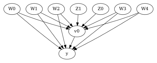
We now input a causal graph in the GML graph format.
[4]:
# With graph
model=CausalModel(
        data = df,
        treatment=data["treatment_name"],
        outcome=data["outcome_name"],
        graph=data["gml_graph"],
        instruments=data["instrument_names"]
        )
[5]:
model.view_model()
[6]:
from IPython.display import Image, display
display(Image(filename="causal_model.png"))
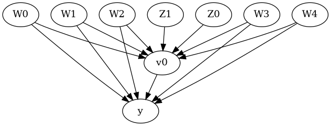
We get a causal graph. Now identification and estimation is done.
[7]:
identified_estimand = model.identify_effect(proceed_when_unidentifiable=True)
print(identified_estimand)
Estimand type: EstimandType.NONPARAMETRIC_ATE

### Estimand : 1
Estimand name: backdoor
Estimand expression:
  d
─────(E[y|W4,W1,W2,W3,W0])
d[v₀]
Estimand assumption 1, Unconfoundedness: If U→{v0} and U→y then P(y|v0,W4,W1,W2,W3,W0,U) = P(y|v0,W4,W1,W2,W3,W0)

### Estimand : 2
Estimand name: iv
Estimand expression:
 ⎡                              -1⎤
 ⎢    d        ⎛    d          ⎞  ⎥
E⎢─────────(y)⋅⎜─────────([v₀])⎟  ⎥
 ⎣d[Z₀  Z₁]    ⎝d[Z₀  Z₁]      ⎠  ⎦
Estimand assumption 1, As-if-random: If U→→y then ¬(U →→{Z0,Z1})
Estimand assumption 2, Exclusion: If we remove {Z0,Z1}→{v0}, then ¬({Z0,Z1}→y)

### Estimand : 3
Estimand name: frontdoor
No such variable(s) found!
Method 1: Propensity Score Stratification#
We will be using propensity scores to stratify units in the data.
[8]:
causal_estimate_strat = model.estimate_effect(identified_estimand,
                                              method_name="backdoor.propensity_score_stratification",
                                              target_units="att")
print(causal_estimate_strat)
print("Causal Estimate is " + str(causal_estimate_strat.value))
*** Causal Estimate ***

## Identified estimand
Estimand type: EstimandType.NONPARAMETRIC_ATE

### Estimand : 1
Estimand name: backdoor
Estimand expression:
  d
─────(E[y|W4,W1,W2,W3,W0])
d[v₀]
Estimand assumption 1, Unconfoundedness: If U→{v0} and U→y then P(y|v0,W4,W1,W2,W3,W0,U) = P(y|v0,W4,W1,W2,W3,W0)

## Realized estimand
b: y~v0+W4+W1+W2+W3+W0
Target units: att

## Estimate
Mean value: 1.0186573191899289

Causal Estimate is 1.0186573191899289
Textual Interpreter#
The textual Interpreter describes (in words) the effect of unit change in the treatment variable on the outcome variable.
[9]:
# Textual Interpreter
interpretation = causal_estimate_strat.interpret(method_name="textual_effect_interpreter")
Increasing the treatment variable(s) [v0] from 0 to 1 causes an increase of 1.0186573191899289 in the expected value of the outcome [['y']], over the data distribution/population represented by the dataset.
Visual Interpreter#
The visual interpreter plots the change in the standardized mean difference (SMD) before and after Propensity Score based adjustment of the dataset. The formula for SMD is given below.
\(SMD = \frac{\bar X_{1} - \bar X_{2}}{\sqrt{(S_{1}^{2} + S_{2}^{2})/2}}\)
Here, \(\bar X_{1}\) and \(\bar X_{2}\) are the sample mean for the treated and control groups.
[10]:
# Visual Interpreter
interpretation = causal_estimate_strat.interpret(method_name="propensity_balance_interpreter")
/home/runner/work/dowhy/dowhy/dowhy/interpreters/propensity_balance_interpreter.py:45: FutureWarning: The provided callable <function mean at 0x7fabcc10fc10> is currently using SeriesGroupBy.mean. In a future version of pandas, the provided callable will be used directly. To keep current behavior pass the string "mean" instead.
  mean_diff = df_long.groupby(self.estimate._treatment_name + ["common_cause_id", "strata"]).agg(
/home/runner/work/dowhy/dowhy/dowhy/interpreters/propensity_balance_interpreter.py:61: FutureWarning: The provided callable <function std at 0x7fabcc10fd30> is currently using SeriesGroupBy.std. In a future version of pandas, the provided callable will be used directly. To keep current behavior pass the string "std" instead.
  stddev_by_w_strata = df_long.groupby(["common_cause_id", "strata"]).agg(stddev=("W", np.std)).reset_index()
/home/runner/work/dowhy/dowhy/dowhy/interpreters/propensity_balance_interpreter.py:67: FutureWarning: The provided callable <function sum at 0x7fabcc10aca0> is currently using SeriesGroupBy.sum. In a future version of pandas, the provided callable will be used directly. To keep current behavior pass the string "sum" instead.
  mean_diff_strata.groupby("common_cause_id").agg(std_mean_diff=("scaled_mean", np.sum)).reset_index()
/home/runner/work/dowhy/dowhy/dowhy/interpreters/propensity_balance_interpreter.py:71: FutureWarning: The provided callable <function mean at 0x7fabcc10fc10> is currently using SeriesGroupBy.mean. In a future version of pandas, the provided callable will be used directly. To keep current behavior pass the string "mean" instead.
  mean_diff_overall = df_long.groupby(self.estimate._treatment_name + ["common_cause_id"]).agg(
/home/runner/work/dowhy/dowhy/dowhy/interpreters/propensity_balance_interpreter.py:78: FutureWarning: The provided callable <function std at 0x7fabcc10fd30> is currently using SeriesGroupBy.std. In a future version of pandas, the provided callable will be used directly. To keep current behavior pass the string "std" instead.
  stddev_overall = df_long.groupby(["common_cause_id"]).agg(stddev=("W", np.std)).reset_index()
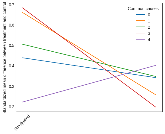
This plot shows how the SMD decreases from the unadjusted to the stratified units.
Method 2: Propensity Score Matching#
We will be using propensity scores to match units in the data.
[11]:
causal_estimate_match = model.estimate_effect(identified_estimand,
                                              method_name="backdoor.propensity_score_matching",
                                              target_units="atc")
print(causal_estimate_match)
print("Causal Estimate is " + str(causal_estimate_match.value))
*** Causal Estimate ***

## Identified estimand
Estimand type: EstimandType.NONPARAMETRIC_ATE

### Estimand : 1
Estimand name: backdoor
Estimand expression:
  d
─────(E[y|W4,W1,W2,W3,W0])
d[v₀]
Estimand assumption 1, Unconfoundedness: If U→{v0} and U→y then P(y|v0,W4,W1,W2,W3,W0,U) = P(y|v0,W4,W1,W2,W3,W0)

## Realized estimand
b: y~v0+W4+W1+W2+W3+W0
Target units: atc

## Estimate
Mean value: 0.9986102796070411

Causal Estimate is 0.9986102796070411
[12]:
# Textual Interpreter
interpretation = causal_estimate_match.interpret(method_name="textual_effect_interpreter")
Increasing the treatment variable(s) [v0] from 0 to 1 causes an increase of 0.9986102796070411 in the expected value of the outcome [['y']], over the data distribution/population represented by the dataset.
Cannot use propensity balance interpretor here since the interpreter method only supports propensity score stratification estimator.
Method 3: Weighting#
We will be using (inverse) propensity scores to assign weights to units in the data. DoWhy supports a few different weighting schemes:
Vanilla Inverse Propensity Score weighting (IPS) (weighting_scheme=”ips_weight”)
Self-normalized IPS weighting (also known as the Hajek estimator) (weighting_scheme=”ips_normalized_weight”)
Stabilized IPS weighting (weighting_scheme = “ips_stabilized_weight”)
[13]:
causal_estimate_ipw = model.estimate_effect(identified_estimand,
                                            method_name="backdoor.propensity_score_weighting",
                                            target_units = "ate",
                                            method_params={"weighting_scheme":"ips_weight"})
print(causal_estimate_ipw)
print("Causal Estimate is " + str(causal_estimate_ipw.value))
*** Causal Estimate ***

## Identified estimand
Estimand type: EstimandType.NONPARAMETRIC_ATE

### Estimand : 1
Estimand name: backdoor
Estimand expression:
  d
─────(E[y|W4,W1,W2,W3,W0])
d[v₀]
Estimand assumption 1, Unconfoundedness: If U→{v0} and U→y then P(y|v0,W4,W1,W2,W3,W0,U) = P(y|v0,W4,W1,W2,W3,W0)

## Realized estimand
b: y~v0+W4+W1+W2+W3+W0
Target units: ate

## Estimate
Mean value: 1.2347572526602477

Causal Estimate is 1.2347572526602477
[14]:
# Textual Interpreter
interpretation = causal_estimate_ipw.interpret(method_name="textual_effect_interpreter")
Increasing the treatment variable(s) [v0] from 0 to 1 causes an increase of 1.2347572526602477 in the expected value of the outcome [['y']], over the data distribution/population represented by the dataset.
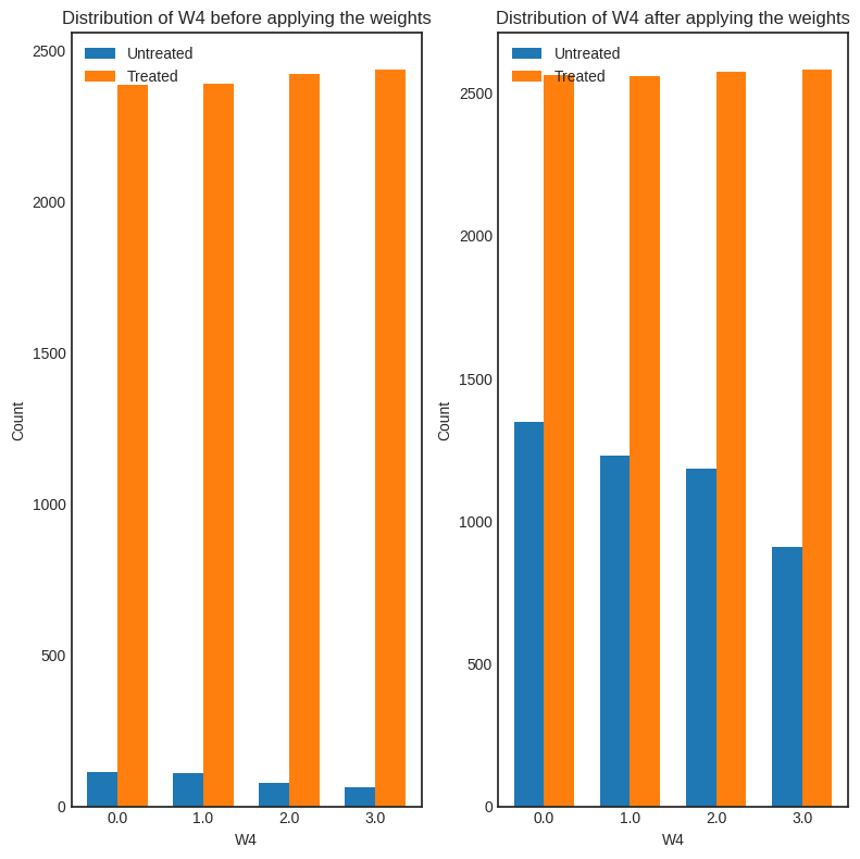
[15]:
interpretation = causal_estimate_ipw.interpret(method_name="confounder_distribution_interpreter", fig_size=(8,8), font_size=12, var_name='W4', var_type='discrete')
/home/runner/work/dowhy/dowhy/dowhy/interpreters/confounder_distribution_interpreter.py:84: FutureWarning: The default of observed=False is deprecated and will be changed to True in a future version of pandas. Pass observed=False to retain current behavior or observed=True to adopt the future default and silence this warning.
  barplot_df_before = df.groupby([self.var_name, treated]).size().reset_index(name="count")
/home/runner/work/dowhy/dowhy/dowhy/interpreters/confounder_distribution_interpreter.py:87: FutureWarning: The default of observed=False is deprecated and will be changed to True in a future version of pandas. Pass observed=False to retain current behavior or observed=True to adopt the future default and silence this warning.
  barplot_df_after = df.groupby([self.var_name, treated]).agg({"weight": np.sum}).reset_index()
/home/runner/work/dowhy/dowhy/dowhy/interpreters/confounder_distribution_interpreter.py:87: FutureWarning: The provided callable <function sum at 0x7fabcc10aca0> is currently using SeriesGroupBy.sum. In a future version of pandas, the provided callable will be used directly. To keep current behavior pass the string "sum" instead.
  barplot_df_after = df.groupby([self.var_name, treated]).agg({"weight": np.sum}).reset_index()
/home/runner/work/dowhy/dowhy/dowhy/interpreters/confounder_distribution_interpreter.py:98: FutureWarning: The default value of observed=False is deprecated and will change to observed=True in a future version of pandas. Specify observed=False to silence this warning and retain the current behavior
  pivoted = plot_df.pivot_table(index=self.var_name, columns=treated, values="count", fill_value=0)
[ ]: