Demo for the DoWhy causal API

We show a simple example of adding a causal extension to any dataframe.

import dowhy.datasets
import dowhy.api

import numpy as np
import pandas as pd

from statsmodels.api import OLS

data = dowhy.datasets.linear_dataset(beta=5,
        num_common_causes=1,
        num_instruments = 0,
        num_samples=1000,
        treatment_is_binary=True)
df = data['df']
df['y'] = df['y'] + np.random.normal(size=len(df)) # Adding noise to data. Without noise, the variance in Y|X, Z is zero, and mcmc fails.
#data['dot_graph'] = 'digraph { v ->y;X0-> v;X0-> y;}'

treatment= data["treatment_name"][0]
outcome = data["outcome_name"][0]
common_cause = data["common_causes_names"][0]
df

	W0	v0	y
0	-1.012777	False	-3.042986
1	0.289858	False	1.112130
2	1.347723	True	8.063621
3	-0.464752	False	-0.189419
4	0.121820	False	-0.439537
...	...	...	...
995	-1.797895	False	-4.532083
996	-1.601010	False	-4.809766
997	-0.639639	False	-1.936961
998	-2.256174	False	-5.319564
999	-0.270505	False	-0.054673

1000 rows × 3 columns

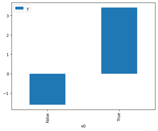
# data['df'] is just a regular pandas.DataFrame
df.causal.do(x=treatment,
                     variable_types={treatment: 'b', outcome: 'c', common_cause: 'c'},
                     outcome=outcome,
                     common_causes=[common_cause],
                     proceed_when_unidentifiable=True).groupby(treatment).mean().plot(y=outcome, kind='bar')

<Axes: xlabel='v0'>

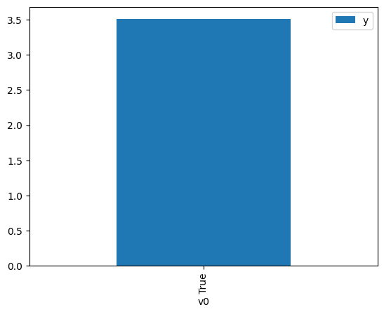
df.causal.do(x={treatment: 1},
              variable_types={treatment:'b', outcome: 'c', common_cause: 'c'},
              outcome=outcome,
              method='weighting',
              common_causes=[common_cause],
              proceed_when_unidentifiable=True).groupby(treatment).mean().plot(y=outcome, kind='bar')

<Axes: xlabel='v0'>

cdf_1 = df.causal.do(x={treatment: 1},
              variable_types={treatment: 'b', outcome: 'c', common_cause: 'c'},
              outcome=outcome,
              dot_graph=data['dot_graph'],
              proceed_when_unidentifiable=True)

cdf_0 = df.causal.do(x={treatment: 0},
              variable_types={treatment: 'b', outcome: 'c', common_cause: 'c'},
              outcome=outcome,
              dot_graph=data['dot_graph'],
              proceed_when_unidentifiable=True)

cdf_0

	W0	v0	y	propensity_score	weight
0	-0.304858	False	-1.448515	0.532390	1.878323
1	-0.625992	False	-2.489382	0.594945	1.680829
2	0.918621	False	2.341392	0.301398	3.317870
3	-0.650677	False	-1.249433	0.599654	1.667629
4	0.232127	False	0.969079	0.426496	2.344690
...	...	...	...	...	...
995	-0.486277	False	-1.746970	0.567984	1.760612
996	-0.994063	False	-0.910734	0.662929	1.508456
997	-0.600021	False	-0.240069	0.589971	1.694998
998	-1.467687	False	-3.689877	0.741164	1.349230
999	0.139491	False	-0.503729	0.444556	2.249433

1000 rows × 5 columns

cdf_1

	W0	v0	y	propensity_score	weight
0	-0.540636	True	3.159776	0.421469	2.372652
1	-0.517413	True	4.373290	0.425967	2.347601
2	-1.011418	True	3.547779	0.334002	2.993996
3	-1.705678	True	-0.387705	0.224299	4.458329
4	-1.809141	True	-0.779102	0.210345	4.754091
...	...	...	...	...	...
995	-0.207755	True	5.120488	0.486822	2.054139
996	-0.597498	True	3.878264	0.410513	2.435976
997	0.806819	True	7.124728	0.679609	1.471435
998	-1.339661	True	3.927840	0.278788	3.586958
999	-2.158812	True	-0.987639	0.167956	5.953941

1000 rows × 5 columns

Comparing the estimate to Linear Regression

First, estimating the effect using the causal data frame, and the 95% confidence interval.

(cdf_1['y'] - cdf_0['y']).mean()

$\displaystyle 5.00995911537052$

1.96*(cdf_1['y'] - cdf_0['y']).std() / np.sqrt(len(df))

$\displaystyle 0.214614822056212$

Comparing to the estimate from OLS.

model = OLS(np.asarray(df[outcome]), np.asarray(df[[common_cause, treatment]], dtype=np.float64))
result = model.fit()
result.summary()

OLS Regression Results

Dep. Variable:	y	R-squared (uncentered):	0.938
Model:	OLS	Adj. R-squared (uncentered):	0.938
Method:	Least Squares	F-statistic:	7593.
Date:	Tue, 05 Sep 2023	Prob (F-statistic):	0.00
Time:	05:11:13	Log-Likelihood:	-1418.2
No. Observations:	1000	AIC:	2840.
Df Residuals:	998	BIC:	2850.
Df Model:	2
Covariance Type:	nonrobust

	coef	std err	t	P>|t|	[0.025	0.975]
x1	2.3582	0.028	85.636	0.000	2.304	2.412
x2	5.0888	0.050	101.283	0.000	4.990	5.187

Omnibus:	5.587	Durbin-Watson:	2.044
Prob(Omnibus):	0.061	Jarque-Bera (JB):	5.476
Skew:	-0.177	Prob(JB):	0.0647
Kurtosis:	3.080	Cond. No.	1.87

Notes:
[1] R² is computed without centering (uncentered) since the model does not contain a constant.
[2] Standard Errors assume that the covariance matrix of the errors is correctly specified.