Demo for the DoWhy causal API

We show a simple example of adding a causal extension to any dataframe.

import dowhy.datasets
import dowhy.api

import numpy as np
import pandas as pd

from statsmodels.api import OLS

data = dowhy.datasets.linear_dataset(beta=5,
        num_common_causes=1,
        num_instruments = 0,
        num_samples=1000,
        treatment_is_binary=True)
df = data['df']
df['y'] = df['y'] + np.random.normal(size=len(df)) # Adding noise to data. Without noise, the variance in Y|X, Z is zero, and mcmc fails.
#data['dot_graph'] = 'digraph { v ->y;X0-> v;X0-> y;}'

treatment= data["treatment_name"][0]
outcome = data["outcome_name"][0]
common_cause = data["common_causes_names"][0]
df

	W0	v0	y
0	-1.085634	False	-4.084557
1	-1.418167	False	-4.159834
2	-1.060908	False	-1.876372
3	-0.040109	True	4.739495
4	-1.135199	False	-2.126015
...	...	...	...
995	0.167694	True	6.002419
996	-1.342202	False	-5.061231
997	-1.115815	False	-4.549248
998	0.224101	False	2.319660
999	-0.559218	False	-1.882604

1000 rows × 3 columns

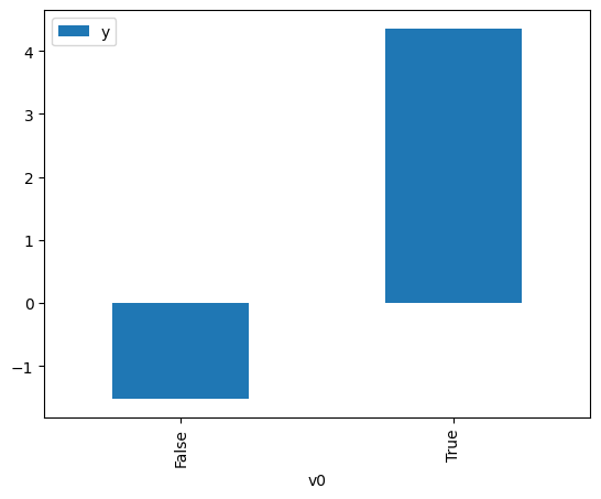
# data['df'] is just a regular pandas.DataFrame
df.causal.do(x=treatment,
                     variable_types={treatment: 'b', outcome: 'c', common_cause: 'c'},
                     outcome=outcome,
                     common_causes=[common_cause],
                     proceed_when_unidentifiable=True).groupby(treatment).mean().plot(y=outcome, kind='bar')

<Axes: xlabel='v0'>

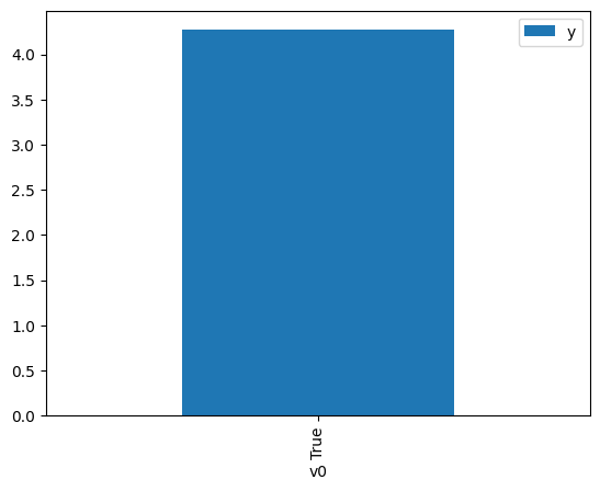
df.causal.do(x={treatment: 1},
              variable_types={treatment:'b', outcome: 'c', common_cause: 'c'},
              outcome=outcome,
              method='weighting',
              common_causes=[common_cause],
              proceed_when_unidentifiable=True).groupby(treatment).mean().plot(y=outcome, kind='bar')

<Axes: xlabel='v0'>

cdf_1 = df.causal.do(x={treatment: 1},
              variable_types={treatment: 'b', outcome: 'c', common_cause: 'c'},
              outcome=outcome,
              dot_graph=data['dot_graph'],
              proceed_when_unidentifiable=True)

cdf_0 = df.causal.do(x={treatment: 0},
              variable_types={treatment: 'b', outcome: 'c', common_cause: 'c'},
              outcome=outcome,
              dot_graph=data['dot_graph'],
              proceed_when_unidentifiable=True)

cdf_0

	W0	v0	y	propensity_score	weight
0	-0.550093	False	-1.532310	0.756892	1.321192
1	-0.722684	False	-1.846021	0.810431	1.233912
2	-1.996264	False	-6.116133	0.977962	1.022534
3	-0.525880	False	-0.314164	0.748614	1.335802
4	-0.668037	False	-3.078179	0.794523	1.258616
...	...	...	...	...	...
995	-2.188685	False	-5.719837	0.984423	1.015824
996	0.607096	False	0.420697	0.270844	3.692155
997	-0.310138	False	-0.762520	0.667047	1.499146
998	-1.141617	False	-4.197842	0.902252	1.108338
999	0.757894	False	1.761406	0.219703	4.551601

1000 rows × 5 columns

cdf_1

	W0	v0	y	propensity_score	weight
0	-0.568209	True	3.579572	0.237036	4.218773
1	-0.506941	True	3.209480	0.257991	3.876099
2	0.701984	True	7.612798	0.762181	1.312024
3	-0.486111	True	4.661744	0.265385	3.768110
4	0.228094	True	5.046634	0.572979	1.745264
...	...	...	...	...	...
995	-0.472540	True	2.449277	0.270274	3.699946
996	-1.012103	True	1.651103	0.120835	8.275773
997	-1.472749	True	0.877186	0.055678	17.960356
998	-0.103875	True	3.710211	0.421676	2.371490
999	-0.375534	True	5.820682	0.306825	3.259191

1000 rows × 5 columns

Comparing the estimate to Linear Regression

First, estimating the effect using the causal data frame, and the 95% confidence interval.

(cdf_1['y'] - cdf_0['y']).mean()

$\displaystyle 5.45773159896272$

1.96*(cdf_1['y'] - cdf_0['y']).std() / np.sqrt(len(df))

$\displaystyle 0.247766786137291$

Comparing to the estimate from OLS.

model = OLS(np.asarray(df[outcome]), np.asarray(df[[common_cause, treatment]], dtype=np.float64))
result = model.fit()
result.summary()

OLS Regression Results

Dep. Variable:	y	R-squared (uncentered):	0.955
Model:	OLS	Adj. R-squared (uncentered):	0.955
Method:	Least Squares	F-statistic:	1.062e+04
Date:	Thu, 03 Aug 2023	Prob (F-statistic):	0.00
Time:	18:29:21	Log-Likelihood:	-1426.4
No. Observations:	1000	AIC:	2857.
Df Residuals:	998	BIC:	2867.
Df Model:	2
Covariance Type:	nonrobust

	coef	std err	t	P>|t|	[0.025	0.975]
x1	2.7773	0.030	93.411	0.000	2.719	2.836
x2	5.0002	0.054	91.951	0.000	4.894	5.107

Omnibus:	2.397	Durbin-Watson:	1.975
Prob(Omnibus):	0.302	Jarque-Bera (JB):	2.464
Skew:	-0.105	Prob(JB):	0.292
Kurtosis:	2.878	Cond. No.	1.89

Notes:
[1] R² is computed without centering (uncentered) since the model does not contain a constant.
[2] Standard Errors assume that the covariance matrix of the errors is correctly specified.