Demo for the DoWhy causal API

We show a simple example of adding a causal extension to any dataframe.

import dowhy.datasets
import dowhy.api
from dowhy.graph import build_graph_from_str

import numpy as np
import pandas as pd

from statsmodels.api import OLS

data = dowhy.datasets.linear_dataset(beta=5,
        num_common_causes=1,
        num_instruments = 0,
        num_samples=1000,
        treatment_is_binary=True)
df = data['df']
df['y'] = df['y'] + np.random.normal(size=len(df)) # Adding noise to data. Without noise, the variance in Y|X, Z is zero, and mcmc fails.
nx_graph = build_graph_from_str(data["dot_graph"])

treatment= data["treatment_name"][0]
outcome = data["outcome_name"][0]
common_cause = data["common_causes_names"][0]
df

	W0	v0	y
0	-1.352371	False	-2.800845
1	1.840101	True	5.312718
2	1.462809	True	5.135988
3	-1.268049	False	-0.090203
4	-1.062236	False	1.062694
...	...	...	...
995	0.278762	False	0.058603
996	1.429788	True	9.476343
997	-2.136987	False	-2.413670
998	-2.070323	False	-1.066857
999	-0.415496	True	3.013789

1000 rows × 3 columns

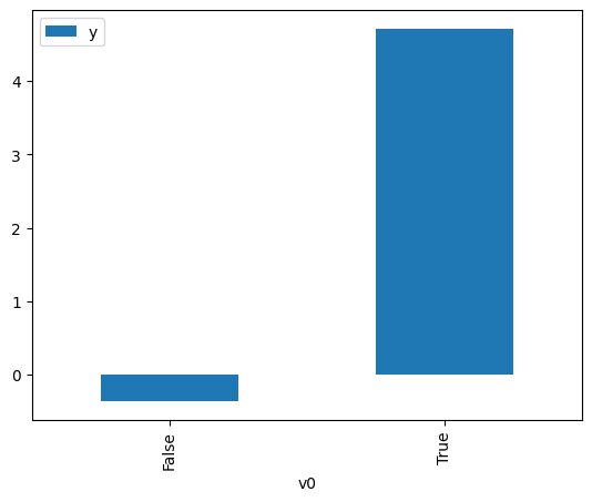
# data['df'] is just a regular pandas.DataFrame
df.causal.do(x=treatment,
             variable_types={treatment: 'b', outcome: 'c', common_cause: 'c'},
             outcome=outcome,
             common_causes=[common_cause],
            ).groupby(treatment).mean().plot(y=outcome, kind='bar')

<Axes: xlabel='v0'>

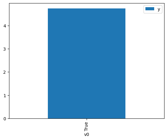
df.causal.do(x={treatment: 1},
              variable_types={treatment:'b', outcome: 'c', common_cause: 'c'},
              outcome=outcome,
              method='weighting',
              common_causes=[common_cause]
              ).groupby(treatment).mean().plot(y=outcome, kind='bar')

<Axes: xlabel='v0'>

cdf_1 = df.causal.do(x={treatment: 1},
              variable_types={treatment: 'b', outcome: 'c', common_cause: 'c'},
              outcome=outcome,
              graph=nx_graph
              )

cdf_0 = df.causal.do(x={treatment: 0},
              variable_types={treatment: 'b', outcome: 'c', common_cause: 'c'},
              outcome=outcome,
              graph=nx_graph
              )

cdf_0

	W0	v0	y	propensity_score	weight
0	2.404146	False	3.487173	0.221540	4.513856
1	-0.119822	False	0.453772	0.542849	1.842132
2	-0.614196	False	0.697349	0.611026	1.636591
3	-0.064320	False	1.124111	0.535044	1.869006
4	-0.137764	False	-1.384972	0.545368	1.833623
...	...	...	...	...	...
995	-0.776681	False	-1.094488	0.632648	1.580659
996	0.397365	False	0.620665	0.469811	2.128515
997	0.713727	False	2.663563	0.425568	2.349803
998	1.595413	False	2.558598	0.310243	3.223276
999	1.712484	False	2.700458	0.296245	3.375582

1000 rows × 5 columns

cdf_1

	W0	v0	y	propensity_score	weight
0	-0.607244	True	3.065915	0.389909	2.564699
1	-0.777414	True	4.223191	0.367256	2.722898
2	-2.025207	True	2.215251	0.222658	4.491188
3	-1.701738	True	1.773618	0.255943	3.907120
4	-0.578541	True	5.247765	0.393781	2.539485
...	...	...	...	...	...
995	0.044282	True	5.576950	0.480276	2.082137
996	-2.149224	True	1.854231	0.210746	4.745046
997	-0.777414	True	4.223191	0.367256	2.722898
998	1.066502	True	5.893722	0.622371	1.606758
999	-0.543172	True	3.854451	0.398569	2.508973

1000 rows × 5 columns

Comparing the estimate to Linear Regression

First, estimating the effect using the causal data frame, and the 95% confidence interval.

(cdf_1['y'] - cdf_0['y']).mean()

$\displaystyle 5.03222846738008$

1.96*(cdf_1['y'] - cdf_0['y']).std() / np.sqrt(len(df))

$\displaystyle 0.125764811665961$

Comparing to the estimate from OLS.

model = OLS(np.asarray(df[outcome]), np.asarray(df[[common_cause, treatment]], dtype=np.float64))
result = model.fit()
result.summary()

OLS Regression Results

Dep. Variable:	y	R-squared (uncentered):	0.929
Model:	OLS	Adj. R-squared (uncentered):	0.928
Method:	Least Squares	F-statistic:	6487.
Date:	Mon, 25 Dec 2023	Prob (F-statistic):	0.00
Time:	07:24:16	Log-Likelihood:	-1372.1
No. Observations:	1000	AIC:	2748.
Df Residuals:	998	BIC:	2758.
Df Model:	2
Covariance Type:	nonrobust

	coef	std err	t	P>|t|	[0.025	0.975]
x1	1.0182	0.028	36.171	0.000	0.963	1.073
x2	5.0284	0.046	108.991	0.000	4.938	5.119

Omnibus:	2.186	Durbin-Watson:	1.932
Prob(Omnibus):	0.335	Jarque-Bera (JB):	2.056
Skew:	0.045	Prob(JB):	0.358
Kurtosis:	2.797	Cond. No.	1.64

Notes:
[1] R² is computed without centering (uncentered) since the model does not contain a constant.
[2] Standard Errors assume that the covariance matrix of the errors is correctly specified.